DC Atmospheric Nitrogen Discharge: Dye Fluorescence

I have been keeping these photo for some time now waiting for the completion of discharge spectra thermal analysis. Since I have been taking forever to do so thanks to the complexity of molecular spectrum; these two photos has been a constant annoyance on my desktop - a reminder of an incomplete work. I have finally decided to release it with some brief information. 

Figure 1: Homemade halogen lightbulb transformer driven flyback DC high-voltage source energizing a multimeter probe. UV emission from corona discharge excites blue fluorescence on paper.

The photo above shows a metallic multimeter probe I've energized with positively rectified high-voltage from a vintage flyback transformer driven by a 12 V halogen lamp high-frequency digital "transformer". Under such high electrical tension, the vertex of the sharp tip have the highest charge density with electric field strength significantly stronger than the dielectric breakdown value of air ~3 million V/m [1, 2]. This causes the tip to glow purple from corona discharge followed by simultaneous release of ozone gas (distinctive musty smell) from the breakdown of oxygen molecules.

Right below the metal tip is a piece of paper acting as electric ground, attracting the positive ions spraying out from the metal tip subsequently causing the paper to glow blue from fluorescence (paper fluoresce because "optical brighteners" has been added). This whole set up was taken with an exposure time of 0.5 second to reveal the corona discharge. The multimeter probe was illuminated briefly by a white L.E.D to cast a shadow, indicating the tip is at a distance away from the paper. 

Figure 2: Vibration energy level of  nitrogen molecule [3]. Major emission lines indicated by red arrow. 

Unfortunately before I am able to measure the output voltage accurately, my last attempt to generate high voltage with similar set-up has resulted permanent damage in the secondary winding of the flyback transformer. My guess is that it has an open-circuit potential around + 20 kV estimated simply based on sharp tipped spark gap distance of 25 mm. The damage was most likely contributed by high current draw (far exceeding 1 mA) without a current-limiting resistor in series with the load (I hooked it up directly to a glow discharge tube) causing a meltdown somewhere within its fine wire coils. 

The lesson: use a ballast resistor for any sort of load.

Figure 3: Emission spectrum of corona discharge. More than 90% light emitted are UVA radiation.

Figure above is the actual dark compensated, 3-second exposure spectrum of the corona discharge taken with OceanOptics USB4000 spectrometer. Even at 3 second exposure (instrumental limit) the data still appears noisy. It was definitely weak light to be picked up by the human eye but the spectrum certainly features at least four peaks within 300 to 400 nm falling under A-subtype UV radiation (keep in mind that ultraviolet light is invisible). 

The four relatively bright emission have wavelengths slightly shorter than peak emission from violet L.E.D but they are less harmful to the eyes compared to emissions from germicidal lamp. All four spectral lines correspond to the second positive system N₂ C → B (vibration bands) of atmospheric nitrogen molecules. More specifically for 337 nm line (important because it will be featured in TEA superluminal sources), the vibration level responsible for the transition is N₂ (C³Π⁺u, v'=0) → (B³Π⁺g, v"=0) of the second positive system [4].

Figure 4a (top): Two glass vials on paper holding water suspension of highlighter pigments, left and right are blue and yellow respectively. Figure 4b (bottom): Long exposure photography shows yellow highlighter dye fluoresce while blue dye remains dark. Notice the blue fluorescence of paper under UVA irradiation.

Now, without anymore further discussions available, I bring up an experiment from the past dealing with fluorescence of highlighter pigments. Earlier, I have tested the dyes and found out the blue highlighter dye does not fluoresce under violet L.E.D. I thought probably light with wavelength shorter than 390 nm might do the work, so I tested the blue dye with UVA emissions of a corona discharge. Not surprisingly, the blue still shows negative response.

REFERENCE

[1] Tipler, Paul A., "College Physics", Worth, 1987, pp.467

[2] Rigden, John S., "Macmillan Encyclopedia of Physics", Simon and Schuster, 1996, pp.353

[3] F. Arqueros, F. Blanco, F. Rosado, "Analysis of the Fluorescence Emission of Atmospheric Nitrogen by Electron Excitation and its Application to Fluorescence Telescopes", New J. Phys., 2009, pp.11

[4] H. Khatun, A.K. Sharma, P.K. Barhai, "Experimental Study of Low-Pressure Nitrogen Dielectric Barrier Discharge", Braz. J. Phys., Vol.40, No. 4, 2010, pp.450 

Crude Plasma Diagnostics for UVC Germicidal Lamp

* This article is closely associated with a previous entry. The author assumes reader understand basic definition of physical plasma as the fourth state of matter.

Figure 1: Applying magnetic field towards the plasma causes its shape to distort due to Lorentz force acting on moving charged particles.

It was a while ago I took a spectrum of the UVC germicidal lamp without its waterproof quartz glass. Its discrete sharp peaks can be described by hallmark of the old quantum theory - light emitted due to electronic transitions between discrete energy levels within the gaseous atoms contained inside the tube. Within the past hundred years, physicists has worked out many useful formulae to relate measurable parameters of a gas discharge spectra such as intensity and its associated wavelength with physical mechanisms that is happening inside the tube at the atomic level. Here, I have worked out some crude but important characterization of the plasma when the UVC germicidal lamp is energized.

Figure 2: Spectrum of UVC germicidal lamp with tagged wavelengths for 17 strong peaks 

After plotting the numerical data into a spectrum (above), I have listed down the wavelength and intensity for 27 individual peaks which I had identified its origin thanks to NIST online database. Interestingly, the peaks was the "fingerprint" of not one but two different chemical elements (as low pressure gas) inside the tube. As mentioned in previous post, the beautiful cyan glow and strong UVC emission at 253.7 nm are the principal character of electrically excited low pressure mercury-vapour, hence finding peaks corresponding to mercury atoms is not surprising. The second interesting element was argon which I presume it was the "filler" noble gas when they used to purge the tube before vacuuming down and filling it up with a small quantity of mercury vapour. All the peaks are of neutral, i.e. Hg (I) and Ar (I) atoms.

Out of 27 peaks, 10 belongs to Hg (I) transitions while the rest are Ar (I). Finding the peaks was easy with common graphing tool (I used Origin 7.0). To make further analysis clear, I shall begin by separating this study into a few components:

1. Calculation of Electron Temperature via Boltzmann Plot

2. Voigt Profile Fitting of Spectral Peak to Determine Broadening Mechanism

3. Estimation of Plasma (absolute) Temperature

4. Comparing Peak Intensity Ratio for Self-Absorption Mechanism

5. Conclusion on Plasma Diagnostics With Respect To Electrical Characteristics

ELECTRON TEMPERATURE AND BOLTZMANN PLOT

You can think of plasma as a "hot soup" of randomly colliding electrons and ions. The electron temperature of plasma allows us to gauge the "hotness" or more specifically the statistical kinetic energy of electrons bumping randomly to each other. Because electrons are so much lighter compared to ions, they transfer energy in different rates when they collide with ions than itself. As such, for the value of electron temperature to stay valid, it is important that the plasma have reached a state where all its particles, i.e. electrons, atoms and ions has reached a common temperature known as Local Thermal Equilibrium (LTE). Otherwise, this physical quantity is known as "excitation temperature".

This temperature can be calculated through the famous Boltzmann plot. In essence, it assumes two emission energy levels of the same atomic population, Ei and Ek are in thermal equilibrium at temperature T, given by:

Equation 1

where N1 and N2 denotes number density and g1 and g2 are the statistical weights respectively. The total number density (I skipped a few algebraic derivation steps) can be simplified to:

Equation 2

At LTE, the intensity for each spectral peak is given by:

 Equation 3

where Aji is the Einstein coefficient for upper transition probability. Rearranging equation 3 by taking natural logarithm on both sides for linearising the expression (y = mx+c) we arrive at:

Equation 4

where the gradient, (-1/kT) tells the electron temperature T, of the plasma. This is the Boltzmann plot where the x and y parameter of this linear expression can be obtained both experimentally (intensities and wavelengths) and from NIST standards (energy levels, Einstein coefficients and statistical weights). 

One interesting outcome for plotting this is that from the data points is that we can determine if the spectrum is "optically thin" through the degree of linearity, i.e. the points coincide a straight line. Optically thick spectra is typically associated with dense plasma where some part of its light has been re-absorbed into the plasma itself, rendering the spectra unreliable for temperature analysis. From tedious work finding all the parameters for Boltzmann plot, I managed to do it for both mercury and argon:

Figure 3: Boltzmann plot for argon lines (top) and mercury lines (bottom). While the data is chaotic for argon's case, data for mercury seems to exhibit linearity where the expected gradient enables calculation of the electron temperature. 

Even though argon has 17 emission lines, it is immediately obvious that the Boltzmann plot for argon lines yields chaotic results for a linear fit. Fortunately, there seems to be a linear relationship for mercury lines and I have used a linear fitting software which gave me a gradient of -1.43 with error of 0.35. This yields electron temperature at (0.699 ± 0.37) eV that is 8112 K for people not in plasma physics and 8384.7 degrees Celsius for non-physicists. The temperature is in the order of magnitude similar to discharge lamps reported in various literature elsewhere. 

PEAK PROFILE FOR BROADENING MECHANISM

The spectrum for plasma (refer to figure 2) contains discrete sharp peaks which I have briefly mentioned as the result of electronic transitions within trillions of atoms of the gas contained in the germicidal lamp. Following the quantum theory, ideally for each electronic transition, the atom emits one particle of light, the photon, with a fixed wavelength and should result an infinitely thin line. However, experiments should find that no matter how "pure" a plasma is, we will always see the peak profile having a broadened "waist", like a mountain. So what was broadening it? 

Broadly, there are three primary mechanisms causing this effect here listed with decreasing significance:

1. Doppler effect coming from light emitted from moving particles within the plasma which reveal itself as spectral line with a Gaussian profile.

2. Stark effect coming from energy levels (especially those close to the continuum) of an atom being "disturbed" by electric fields of nearby moving ions and/or externally applied E-field, this effect reveal itself in spectral line of Lorenzian profile. 

3. Intrinsic property of quantum mechanics itself. i.e. the Heisenberg Uncertainty Principle, which states that any electrically excited atoms having a finite lifetime will have slight indeterminate energy level, causing the light emitted from atoms having so slightly a shorter or longer wavelengths with one another. An effect I believe too insignificant to observe based on the resolution of our experiment set-up.

For simplicity sake, I have chosen the brightest peak of the spectrum, i.e. the line at 253.7 nm for profile analysis. As we magnify the wavelength scale, we will see the "line-like spike" resolve into a "mountain". There are a few types of fitting available to extract information regarding its shape. For further analysis, I used a combination of both Gaussian and Lorenzian profile fitting - the Voigt profile. 

Figure 4: Voigt profile fitting for the brightest spectral peak at 253.7 nm. Red line indicates the fitting.

Using a Voigt fitting, Origin 7 provides me two w parameters for defining the typology of the "mountain" shape. A ratio of wG and wL (0.00381/1.91006) gives us 0.002 which is significantly less than 0.5 - the threshold for Lorenzian profile, so Gaussian it is.      

Figure 5: First order derivative of fitted Voigt profile. The peaks enables calculation of FWHM value.

Identifying the peak having a Gaussian profile has an advantage. Other than confirming the dominant broadening mechanism as the result of Doppler effect, a simple equation based on Maxwellian distribution can be used to estimate the absolute temperature of the plasma by knowing the profile's full wave half maximum (FWHM) value. We will discuss that in the next sub-chapter but for the moment, I have worked out the FWHM via first order derivative of said Voigt profile. 

The positive and negative peaks of Voigt derivative correspond to the half-width value Δλ1/2, where |254.28 - 252.51| = 1.77 nm.   

ESTIMATION OF PLASMA TEMPERATURE 

As mentioned before, to characterize a plasma which composed of different types of particles, have to account two different temperatures. While we have characterized the electron temperature with Boltzmann plot, there is another class of particles - ions, which are heavier and moves slower relative to electrons and their temperature can be related to the absolute temperature of the plasma based on FWHM for Doppler broadening given by:

Δλ1/2 = 2λ SQRT (2kT ln 2 / mc^2)

Equation 5

where λ is the peak wavelength, m is the atomic mass and c is the speed of light. T is the absolute temperature where by rearranging the equation, I have calculated it to be 1.84E10 degree Kelvin. Which is rather nonsensical. For comparable results with our previously obtained electron temperature (plasma temperature should be slightly "less hotter" than electron temperature but LTE demands them to be as close as possible) the FWHM value should be in the order of 0.001 nm, which is far beyond the resolving capabilities of my spectrometer set-up. 

I would argue such absurdities are due to equation 5, which depends heavily on the FWHM value which was limited experimentally by my spectrometer slit width, not until we analyze FWHM for each 27 peaks using precision spectrometer (which is quite a lot of work), I cannot be convinced that the absolute temperature falls in that order of magnitude. Naturally, because the plasma temperature differs so greatly with the electron temperature, I cannot conclude the plasma is even in LTE. 

PEAK INTENSITY RATIO FOR SELF-ABSORPTION MECHANISM

There is however another way to determine the "usability" of the spectrum by finding its optical "thickness" with experimental intensity ratio between two emission lines that has the same upper energy level, described by:

Equation 6

we can eliminate the exponential term since E2 = E1, and therefore leads to: 

Equation 7

where the left hand side (L.H.S) can be obtained via experiment intensity and right hand side (R.H.S) through NIST standards. With that, I have came to using three Hg (I) lines of 404.11 nm, 435.34 nm and 545.94 nm having identical upper energy level at 62350.325 cm^-1 corresponding to electron shell 3s at 5d(10)6s7s configuration, calculated their LHS and RHS values to be 2.57 against 1.43 and 3.57 against 2.46. Both differ by at least 1.1 suggesting optically thick plasma. This can be interpreted as self-absorption of photons by the atoms inside the plasma and the rate of absorption differs between different spectral lines depending on factors like energy level lifetime and charge densities etc.

CONCLUSION

To be honest, eventually diagnosing the plasma as optically thick was rather disappointing considering the amount of work spent on gathering spectral data from NIST and the associated analysis. Nonetheless we learned that the plasma confined within the germicidal lamp's quartz tube contains argon. Even though no conclusion can be drawn on the state of LTE for the plasma, the electron "excitation" temperature was found to be in the order of magnitude expected for a discharge lamp, that is at around 8000 K based on Boltzmann plot. The plasma temperature was found to be in the order of 10,000,000,000 K is unrealistic, but it was due to experimental limitation vis-a-vis the design of the spectrometer (thus limiting the FWHM resolution). It could also be due to some other broadening mechanisms which I have overlooked. 

On optical thickness, I am tempted to suggest the difference between LHS and RHS terms from equation 7 arise from self-absorption are due to the electrical characteristics of the plasma. The germicidal lamp is most probably energized by alternating voltages which cause the particles in the plasma to "move" differently when it is energized by static DC sources. To understand these character of a plasma in detail, I recommend further work on a system that enables me to fix the state of vacuum and gas inside a chamber where we can manipulating the electrical properties of plasma to study its spectral changes although such work will be painstakingly time consuming. 

REFERENCES
[1] N.M. Shaikh, B. Rashid, S. Hafeez, Y Jamil and M.A. Baig, "Measuremement of Electron Density and Temperature of Laser Induced Zinc Plasma", 2006, J. Phys D: Appl. Phys., pp.1384
[2] C. Aragon, J.A. Aguilera, "Characterization of Laser Induced Plasmas by Optical Emission Spectroscopy: A Review of Experiments and Methods", 2008, Spectrochimica Acta B, pp.893
[3] A.D.Giacomo, V.A.Shakhatov, O.De Pascale, "Optical Emission Spectroscopy and Modeling of Plasma Produced by Laser Ablation of Titanium Oxides", 2001, Spectrochimica Acta B, pp.753

Experimental Proof of Planck's Constant using LED

I received a lovely book as a birthday gift from a friend whom I told once I was so keen to get myself a copy but couldn't afford at that time. Authored by a father-daughter duo, they are more than simple enthusiast for reproducing some of the greatest work in 20th century physics. Exploring Quantum Physics through Hands-on Projects really provides all the little ideas (and some not so little) for the home-experimenter to verify some of the important works in physics which has earned its pioneers their Nobel prize.

In this article, I'll give an account of an experiment I've done according to that was described in chapter 4. The basic principle discussed was quantization which the authors called "the core for quantum physics". In it, they described a simple but effective "visualization" of Planck's constant at work using LED of different colours. 

A simple circuit can visualize Planck's constant at work - proving quantization as part of nature's behavior.  

The theory suggest that a single coloured LED (not white) emit almost (but not quite) monochromatic light. Assuming they do, the energy required to generate particles of light (photons) streaming out of the LED, have energy described by simple equation:

E = hf = (hc)/wavelength , c is speed of light in vacuum

Which states the energy, E, of a single particle of light is directly proportional to its frequency under a physical constant called the Planck's constant, h. 

Now because the colour of light is associated with its wavelength (and hence frequency), not surprising it will require increasing amount of energy to power LED that generates light with short wavelength (or high frequency). The Prutchi duo indeed suggest the constant h can be approximated by measuring the wavelength (or frequency) of light and voltage required to "start" LEDs. This is only true by assuming the energy of the photon is a direct consequence of the electrons transit from a higher level to a lower level corresponding to the materials inside the LED:

eV = hf = (hc)/wavelength , assuming E = eV

where e is the charge of an electron and V is the voltage required to "switch on" the LED. 

I have five LED of different colour which I have their wavelength measured using an Ocean Optics USB spectrometer. The results were normalized for all the LED emissions and graphically represented below:

The spectral profile of LEDs. They emit light with one peak wavelength corresponding to their colour.  

Specifically, the spectral emission peaks are 631 nm, 595 nm, 561 nm, 527 nm and 456 nm giving uncertainty of 2 nm for spectrometer calibration. The wavelengths correspond to their appearance: red, orange, yellow-green, green and blue respectively. 

By connecting the LED in series with a potentiometer powered by a 9 V battery, the "switch on voltage" can be measured by placing a multimeter probe between the LED electrodes while adjusting the potentiometer such that the LED start to emit light. 

When I did the experiment, I found a major flaw in its argument. The authors of the book themselves explained that this method can only approximate the constant h due to the very nature of LED themselves. To say light emitted from electron transition due to externally applied electric potential inside the "active region" of the LED is an oversimplification of the real case. 

1. The emission of light, as I found, happens even in as low as 0.07 V. As long as the LED is properly connected to their terminals (sign not reversed), a slight potential difference across it will cause a tiny current flowing through the diode which cause it to emits light. 

2. When the voltage is increased to about 1 V, the LED gets progressive brighter and at 1.75 V for LED designated "red", the brightness suddenly increased indicating "switching on". This sudden "switch on" voltage varies with LED of different colour and it is the parameter which we measure. 

The two points above actually describes the character of a semiconductor diode which I will not explain its operating mechanism in detail. Briefly, the wavelength of light emitted is actually dependent on the band-gap energetics of the materials between a p-n junction. The voltage I measured was actually the "forward bias voltage drop, Vd" corresponding to the point when the voltage-current curve starts to exhibit exponential behavior. 

Photograph taken by myself showing the "active region" in a green LED. Notice the tiny bright cubic crystal sitting on the reflective cavity supported by the cathode anvil "flag". Two thin wires connects the crystal are the cathode and anode providing energy (electric potential) to create light.

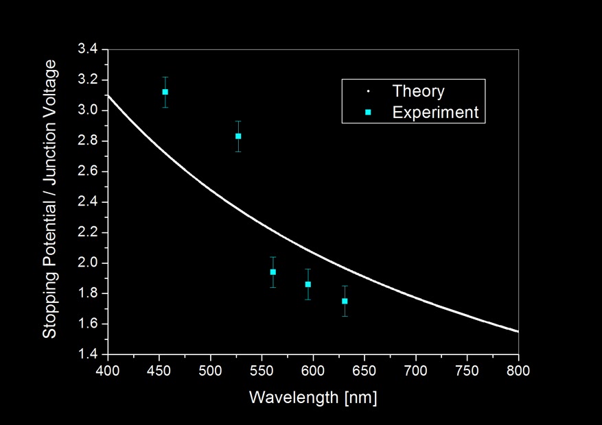
Nevertheless, I tabulated the data and plot a graph that include both a "theoretical" computation assuming [eV = (hc)/wavelength] and "experiment" points:

Notice how far the experiment results deviates from theory which assumes energy needed to generate light, E = eV even after including measurement uncertainties. But because 5 experiment points cannot statistically justify the trend, I calculated the Planck's constant, h, based on the result obtained from the 5 LEDs.

The average turns out actually not bad when compared to the actual value of Planck's constant: 6.626E−34 Js. Which differs only about 0.2% considering an experiment based on so many assumptions. It need to be noted that this apparently "good" result is also derived from statistics (since we averaged it), so given if we have more LEDs which emits light in wavelength other than the five I currently have, the "new" averaged result might not be so beautiful. 

This experiment tells us one important thing: that quantization of energy in the form of light, is detectable even in a slightly complicated solid-state system such as the LED. Different colours of light indicated by its frequency regardless of where it comes from, whether from our star, the lamp in our house to the screen we touch can be regarded as little "packets" of energy emitted from them. Each little "packet" is an energy signature that is in the multiple of Planck's constant. They typically enters our eye in huge numbers having different energy individually for different colours. These little particles or "corpuscles" as Sir Isaac Newton calls it, brought us a beautiful universe through a sensory perception we call sight. 

Fluorescence in Highlighter Pigments

It took me a while to publish these new photographs thanks to work and all those things associated with bad publications. Luckily, my homemade set-ups never stopped during these times and I now managed some time to whip up a quick but interesting post. 

An acrylic carrom striker puck imbued with fluorescent material glows green when exposed to near ultraviolet light. The light source used for this photo was from a commecially inexpensive near-violet LED.

About a month ago, I received a complimentary 5-colour-in-1 highlighter as a door gift from an exhibition. Since I only use yellow and blue for all my highlighting jobs, I decided to use the pigments contained within these highlighters for the so-called UV photography. There are a few types of UV photography techniques but this article in particular focuses on a phenomena called "fluorescence". 

Fluorescence is a form of luminescence. An object is fluorescent if it emits light after absorption of light in another wavelength. Typically, light of shorter wavelength will be absorbed by a fluorescent material and re-emitted as light in longer wavelength. Fluorescent is familiar to us. Most people know shining ultraviolet (shorter wavelength) from commonly available "black-light" on bank notes will reveal strips of glowing colours typically red or orange (longer wavelength). These strips are essentially fluorescent paints that was printed on bank-notes for the purpose counterfeit identification.

Now as far as I am familiar with highlighters, I know they contain fluorescent pigments to exhibit bright colours. Pyranine is a known fluorescent dye that was added into yellow highlighters but I was curious to know what pigment is responsible for other colours or if they could fluoresce at all. So I disassembled the new 5-in-1 highlighter, removed the felt tip and washed all the spongy core with 20 ml of deionized water. It appears water is an excellent solvent for all the colours and I kept them separated with a glass vial for a while. 

Lately I came across a very cheap source of ultraviolet light. Apparently near UV light sources was already introduced commercially in the form of inexpensive light emitting diodes. These LED typically made from mixing different portions of Gallium Nitride (GaN) and Indium Nitride (InN) are able to release continuous near-violet UV light peaked at 390 nm. I bought my light source with MYR 5 from a night market and was able to demonstrate the following:

One colour did not glow under UV. Does it require light of a shorter wavelength to exhibit fluorescence? 

The picture above shows 5 different highlighter colours mentioned earlier. They were diluted to approximately the same concentration to about 3 ml each colour and kept in glass sample bottles (top). When shined with near violet light, only 4 colours appears to fluoresce (bottom). Perhaps blue highlighter needed another light source with wavelength shorter than 390 nm to cause it fluoresce? Needless to say, the photograph describes the relative intensity of fluorescence emission from the other 4 dyes pretty well. Based on visual observation, the green dye could actually share same fluorescent material with yellow. But we will never truly know unless we get a spectroscopic data from these samples. 

Quantum Quotes

The quantum mechanics solution, that is, "Don't worry!" We can't measure it, is logical enough, but not satisfying to most human minds, which strive to understand the details of the world around us. For some tortured souls, the quantum unknowable-ability (Heisenberg's uncertainty principle) is still too high a price to pay.

Our Defense: This is the only theory we know now that works. Ugly but it works.



- adapted and edited from "The God Particle" 1993 L. Lederman

A little thing about waves

Adapted from Wikimedia. Translated and edited by myself.

The red curvy line is a representation of wave.

All the other components are noted down.

The period of the wave (wave period) is usually denoted as the symbol T.

The wavelength is usually denoted with the greek letter lambda (λ).

The frequency of a wave is given by the formula:

Where the symbol f is the frequency.

*Note that frequency is the reciprocal of the wave period.*

The unit for frequency is Hertz. (Hz)

In short, the shorter the wavelength means higher frequency (more waves in a second) and if the wavelength is longer, it means it has less waves in a second.

For musicians,they see frequency as pitch. Everytime when they play a tone, it reprisents a note with a specific frequency. For example:

Start with the middle C in piano, and it goes C, D, E, F, G, A, B, C. This is called an octave. As you press the keys starting from the middle C to the next adjacent keys, you are actually listening to the a note with a higher frequency each time you press it.

So, each time you press the adjacent keys, all you hear is the note with a higher pitch.

Click here for a more details about waves. (high school level)